

Language:
Español
Themes:
Introduction
Principle
Timing
Notation
Chirps
Exceptions
Statistics
Mailing list
Links
|
The ionosonde transmitter in fact sends a continuous carrier, but with
smoothly changing frequency, at a fixed but accurate rate (in the case of
most chirp sounders we use, with increasing frequency at 100 kHz/second).
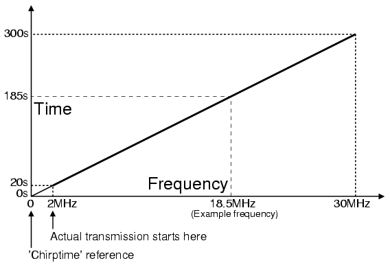
Knowing the chirp rate of the transmission, and what frequency the chirp is being received on, one can work out the nominal "chirp time" at which the received signal started at zero - by simply counting back at 100 kHz/second. |
In the plot, we see that an example frequency of 18.5 MHz, corresponds to a 'chirptime' of 185 seconds (18.5/0.1), meaning that at 18.5 MHz, the chirp will be heard 185s later than the characteristic time for that station.
Peter's design uses the special chirped filter previously described, with properties not attainable with a conventional filter, and so is able to detect the transmissions with 0.66 ms time resolution, and with very narrow bandwidth that provides high sensitivity.
There are two useful advantages of this chirped filter technique:
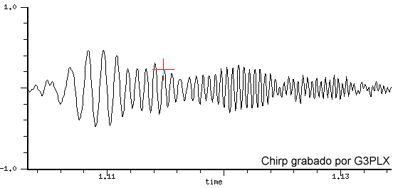
The graph corresponding to the audio of the chirp in the text |
In the case of conventional chirped ionosondes, the receiver is more
conventional, but follows (tracks) its matching transmitter throughout the
HF spectrum. In this passive sounding project, the receiver tracks many
different transmitters using the chirped filter, but only over the width of
an SSB receiver bandpass - about 2.4 kHz - since the receiver frequency is
fixed. This approach is more than sufficient for sensitive single frequency
measurements. You simply set the receiver frequency to suit the band you
wish to know about. Download and listen to a typical chirp received in a 2.4 kHz bandwidth. |
| Copyright Murray Greenman and Peter Martinez, 1999 - 2003 |