
Language:
Español
Themes:
Introduction
Principle
Timing
Notation
Chirps
Exceptions
Statistics
Mailing list
Links
The transmissions used by this project are chirped sounders which transmit a continuously swept signal, nominally from 0 to 30 MHz, at a constant rate of 100 kHz/second. Most of these sounders are commercial and research transmissions for vertical or oblique ionospheric sounding purposes. Some are probably military sounders with a similar purpose.
Note that there are a number of frequencies regularly excluded from the scan, to avoid interference with essential services.
Once the capabilities of this passive sounding technique are understood, and of course if the results of this research experiment prove to be both useful and achievable, it may be possible to develop a system which will enable anyone with an interest in HF propagation to study it in real time with a minimum of equipment and expense - for example using nothing more than a PC with sound card. Perferably, one reference sounder could be used to calibrate reception of others, avoiding the need for an expensive high precision time reference.
There are more or less three phases to this project envisaged:
Several sounder transmissions were identified and their locations discovered by hyperbolic triangulation (measurement of arrival times at different locations and plotting lines of equal delay). Improved tracking of sounders with different chirp periods, improved time resolution and simpler setup, clock synchonisation and system calibration were perceived as the main areas for improvement.
Four observing stations took part in Phase I - one in the UK, one in New Zealand, one each in North and South America. Three of these were capable of high precision time measurement. Stations were in many cases able to receive the same signals, thus making distance measurements possible. Both long and short path transmissions could be identified by timing, and on occasions it was possible to resolve long path and short path signals simultaneously. On a few occasions round-the-world delays were detected.

Better data analysis allows more accurate delay measurements to be made, making possible the identification of individual propagation paths. At present five stations are equipped for Phase II sounding, although it is hoped that other stations with a better geographic spread will take part. With observers widely spread in this way, more accurate triangulation of the sounder sites is possible, and more opportunities to study sounders at more than one site will occur. This is especially true of the more difficult observations involving sounders that either drift in time, jump in reference time, can only be heard in some locations, or are not available continuously. An army of "chirp spotters" could help solve these problems.
If the transmitter and receiver are in fixed locations, you would expect this delay to be constant. However, it is not, and this variation is the principle on which this project is based. The arrival time of the signal will depend on which way around the world it went, how many times it bounced off the ionosphere and the earth, and which ionospheric layers were involved.
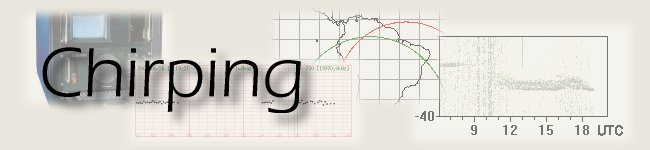
An explanation of the above image is in order. This graph is called a "waterfall", a type of ionogram where the image axes are both time - horizontally in UTC hours (time of day), and vertically in milliseconds, the delay time from some fixed reference point. Since it is not practical to display more than a short period of time vertically with high resolution, the vertical size is limited to ±40 ms (Phase I) or +150ms (Phase II). The image displays the strength of the signal during the receiving "window", using white for no signal, and black for very strong signals. 256 grey levels are displayed, 0.25dB per step, over a range of 64 dB. Imagine that a waterfall is set to a time of 2.5 seconds, with a period of 300 seconds (five minutes). Any signal that appears within 40ms of the UTC five minute points plus 2.5 seconds (00:02.5, 05:02.5 minutes:seconds etc) will be displayed in the waterfall window. This technique is extremely sensitive, as no digital detection process is involved - interpretation is left to the eye.
Unlike most examples shown, the image immediately above shows a constant horizontal line - this is because the transmitter was within groundwave range of the receiver. Much of the day, this is the only signal received; however, between 0600 and 2100 UTC, faint lines first with decreasing and later increasing delay appear. These are caused by scatter to the receiving site from an ionospheric skip occuring to some other part of the world. As the skip zone moves closer, the delay is reduced. The signal suddenly becomes very strong and with a stable short delay between 1200 and 1900 UTC. This is the F layer reflection which occurs during daytime, where the transmitted signal is reflected from the ionosphere and directly received at the observing receiver. The additional delay (i.e. the time later than the ground wave arrival time) is an indirect measure of the height of the reflective layer. If you look closely, you can see that there are actually two separate lines between 1200 and 1900 UTC, the ground wave signal and the F-layer skip signal. The fuzzy stuff with longer delays above these strong lines come about because the reflective layer is diffuse, causing some diffraction (scatter), which you might liken to the fuzziness of a rainbow.
| Copyright Murray Greenman and Peter Martinez, 1999 - 2003 |